Microsoft, OpenAI and the future
Since 2016, Microsoft has strived to become an AI powerhouse on the global scale. The goal is to transform Azure into an artificial intelligence augmented machine with superlative capabilities. To this end, they partnered with OpenAI to build their infrastructure and democratize data. As of now, there are several promising results. Such as the infrastructure used by the OpenAI to train its breakthrough models, deployed in Azure to power category-defining AI products like GitHub Copilot, DALL·E 2, and ChatGPT. And Microsoft is not shy about gloating about their progress.
Recently, BitPeak representatives were invited to an event, titled “Azure and OpenAI: Partners in transforming the world with AI”. In this article we will share with you the key points of the Webinar, such as Microsoft strategy, established implementations and use cases, as well as a quick peak into the future of GPT-4.
So, if you are interested in AI, as you should be, you are in luck! Without further ado – let us dive in.
The Microsoft strategy and investments
General Overview of the Strategy
The hosts started strong and put emphasis on the necessity of investments in AI for companies that do not want to be left behind, as constant development creates pressure to progress or become uncompetitive. It was quite an obvious prelude for further promotion of Microsoft’s product, but the sentiment itself is not wrong. AI has come to the mainstream, with decently reliable results and cost-efficiency – and the world is riding on its wave.
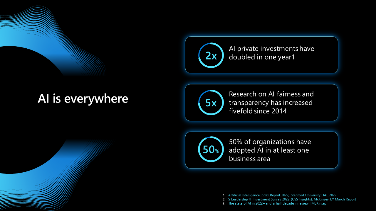
A slide from MS presentation representing the importance of the AI
In its 2022 report about AI, creatively titled “The state of AI in 2022—and a half decade in review” McKinsey supports this conclusion and gives their own insights about the future of artificial intelligence. Unfortunately for all the Luddites, the future with AI powered toasters and/or Skynet is confidently coming our way.
So, how does Microsoft prepare for the coming of our future computer overlords? The answer is simple:
- Research & Technology
- Partnerships
- Ethical guidelines
Research & Technology
The obvious Microsoft flagship is the ChatGPT which conquered the globe in lightning-fast time, reaching 100M users in just two months. In comparison, Facebook took 4.5 years to do the same. The chatbot won the minds and hearts through a combination of its ability to conduct nearly human-like conversations, provide code snippets and explanations, as well as very confidently state very incorrect information. And those are some very human competencies that not every person I know possesses.
But, jokes aside, why is ChatGPT so special and different from other chatbots? The concept itself is not new. However, as demonstrated during the webinar, you can ask it to create a meal plan for a particular family with concrete specifications such as portions, cooking style and nutrition. The bot will create (not paste!) such a plan for you and even provide a shopping list if asked. The list may be wrong the first time, but after some prodding you will get what you need and be ready to go to the nearest supermarket.
The example shows that not only does the AI have some real day-to-day uses, not only can it correct itself (or at least provide the second most probable answer based on its parameters), but also provide assistance in a broad range of topics with various capabilities. But, after knowing “why”, let us look closer at “how”.
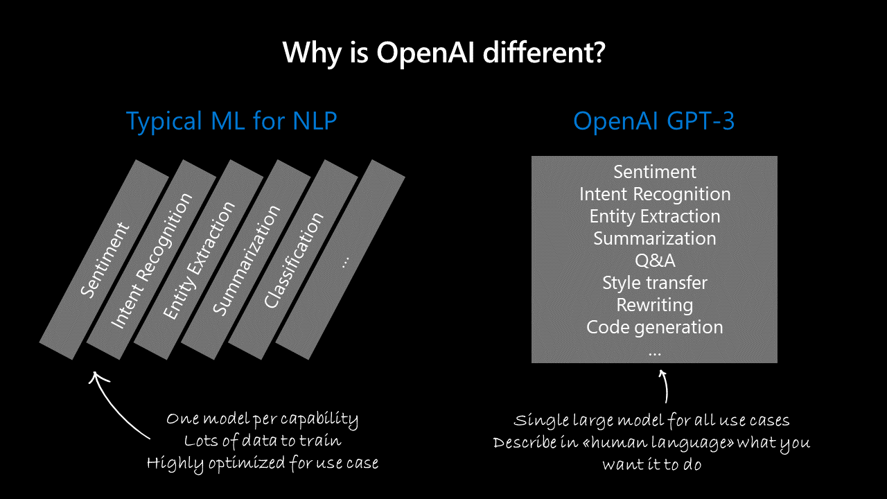 ChatGPT – one model to rule them all
The first part is its architecture. ChatGPT is a single model with multiple capabilities, often referred to as a „single model for multiple tasks”. This is the result of its underlying architecture and training methodology. Such an approach stands in contrast to the traditional solutions, which involve training separate models for each task. But how does it work exactly?
Transfer learning: ChatGPT leverages transfer learning, where it is pretrained on a large corpus of diverse text data, gaining a general understanding of language, facts, and reasoning abilities. This pretraining step enables the model to learn a wide range of features and patterns, which can be fine-tuned for specific tasks. The shared knowledge learned during pretraining allows the model to be flexible and adapt to various tasks without the need for individual task-specific models.
Zero-shot learning: Owing to its extensive pretraining, ChatGPT possesses the ability to perform zero-shot learning in which the model is trained on a set of labeled examples, but is then evaluated on a set of unseen examples that belong to new classes or concepts. This means it can handle tasks it has not been explicitly trained for, using only the knowledge acquired during pretraining. To achieve this, zero-shot learning relies on the use of semantic embeddings, which represent objects or concepts in a continuous vector space. By using these embeddings, the model can generalize from known classes to new classes based on their similarity in the vector space.
Few-shot learning: ChatGPT can also engage in few-shot learning, where it can learn to perform a new task with just a few examples. In this setting, the model is provided with examples in the form of a prompt, which helps it understand the task’s context and requirements. To achieve this, few-shot learning typically employs techniques like transfer learning, meta-learning, and episodic training. Transfer learning involves adapting a pre-trained model to a new task with limited data, while meta-learning involves training a model to learn how to learn new tasks quickly.
Thanks to this approach chatbot is more efficient when it comes to allocating resources, simpler to deploy, better at generalization and adaptation to new tasks, easier to maintain and able to find and use synergies between its capabilities. Why do other AI models either do not use this approach or are not as proficient in it?
The answer is simple – resources. ChatGPT benefits from an enormous amount of resources, both when it comes to infrastructure that supports its capabilities and the sourcing and parsing of training data.
But simple answers are usually not enough. Below are a few more tricks that the AI uses to answer questions ranging from Bar Exam tasks to trivia from the Eighties Show.
Safety: To increase safety, OpenAI employs Reinforcement Learning from Human Feedback (RLHF). During the fine-tuning process, an initial model is created using supervised fine-tuning with a dataset of conversations where human AI trainers provide responses. This dataset is then mixed with the InstructGPT dataset transformed into a dialog format. To create a reward model for reinforcement learning, AI trainers rank different model responses based on quality. The model is then fine-tuned using Proximal Policy Optimization, with this process iteratively repeated to improve safety.
Fine-tuning: Fine-tuning is achieved through a two-step process: pretraining and supervised fine-tuning. During pretraining, the model learns from a massive corpus of text, gaining a general understanding of language, facts, and reasoning abilities. In the supervised fine-tuning stage, custom datasets are created by OpenAI with the help of human AI trainers who engage in conversations and provide suitable responses. The model then fine-tunes its understanding by learning from these responses, improving its contextual understanding and coherence.
Scaling: Scaling is accomplished primarily by increasing the number of parameters in the model. ChatGPT in its newest iteration has billions of parameters that allow it to learn more complex patterns and relationships within the training data. The transformer architecture enables efficient scaling by leveraging parallelization and distributed computing, allowing the model to process vast amounts of data efficiently.
Reduced prompt bias: To reduce prompt bias, OpenAI explores techniques such as rule-based rewards, where biases in model-generated content are penalized. Another approach is to use counterfactual data augmentation, which involves creating variations of the same prompt and training the model on these diverse prompts to produce more consistent responses.
Transformer architecture: The transformer architecture, introduced by Vaswani et al. in 2017, is the foundation of GPT-4 and other state-of-the-art language models. Key features of this architecture include:
- Self-attention mechanism: Transformers use a self-attention mechanism that allows the model to weigh different parts of the input sequence and focus on contextually relevant parts when generating output.
- Positional encoding: Transformers do not have an inherent sense of sequence order. Positional encoding is used to inject information about the position of tokens in the input sequence, ensuring the model understands the order of words.
- Layer normalization: This technique is used to stabilize and accelerate the training of deep neural networks by normalizing the input across layers.
- Multi-head attention: This mechanism enables the model to focus on different parts of the input sequence simultaneously, learning multiple contextually relevant relationships in the data.
- Feed-forward layers: These layers, used after the multi-head attention mechanism, consist of fully connected networks that help in learning non-linear relationships between input tokens.
By leveraging these advanced features, the transformer architecture empowers ChatGPT to generate more contextually accurate, coherent, and human-like text compared to other AI models.
Partnerships
To establish and retain a dominant position in the AI tech-sphere, Microsoft has been actively pursuing strategic partnerships with leading research institutions, startups, and other technology companies. These alliances enable Microsoft to tap into external expertise, share knowledge, and jointly develop cutting-edge AI solutions, broadening their offer of AI-augmented services and tailoring them to their infrastructure. The most important partner is obviously OpenAI, which together with Microsoft develops four main models.
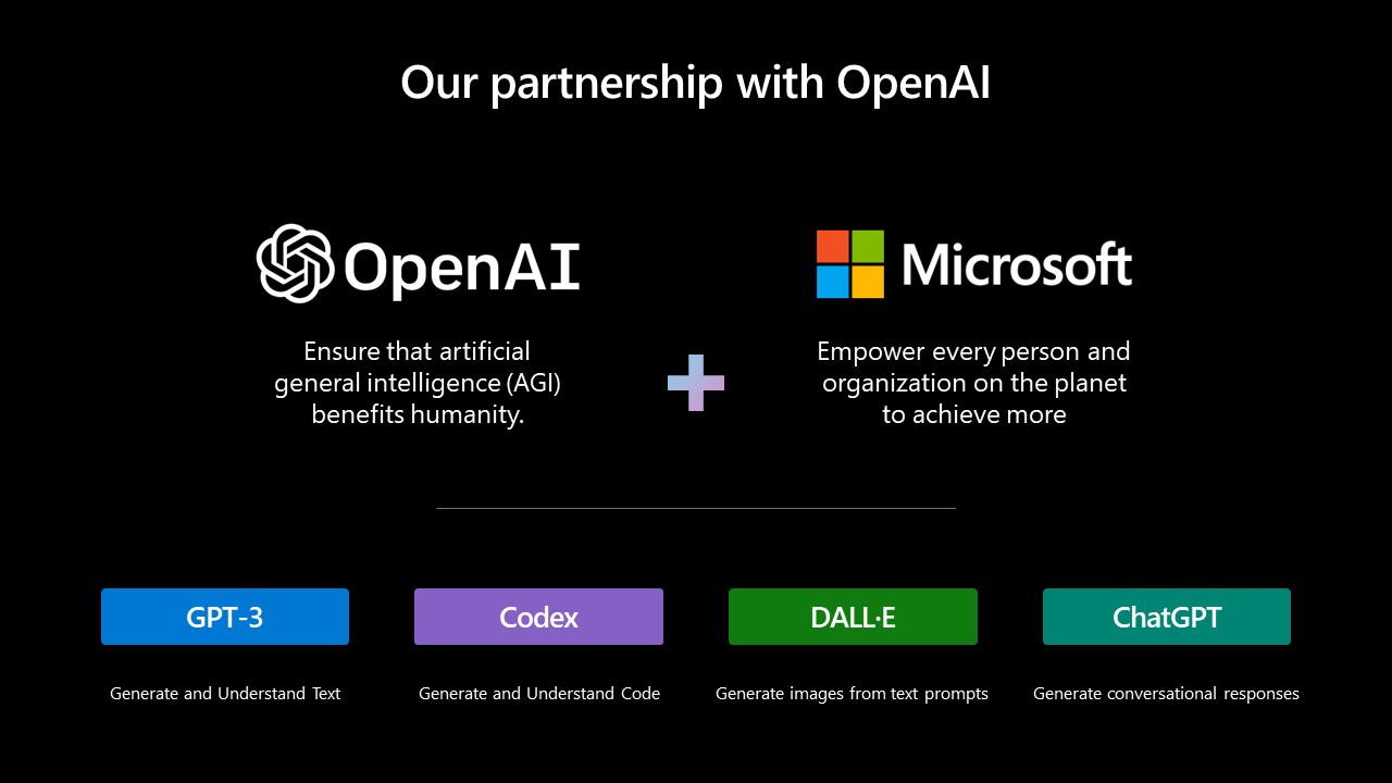
Joint mission and results of the partnership
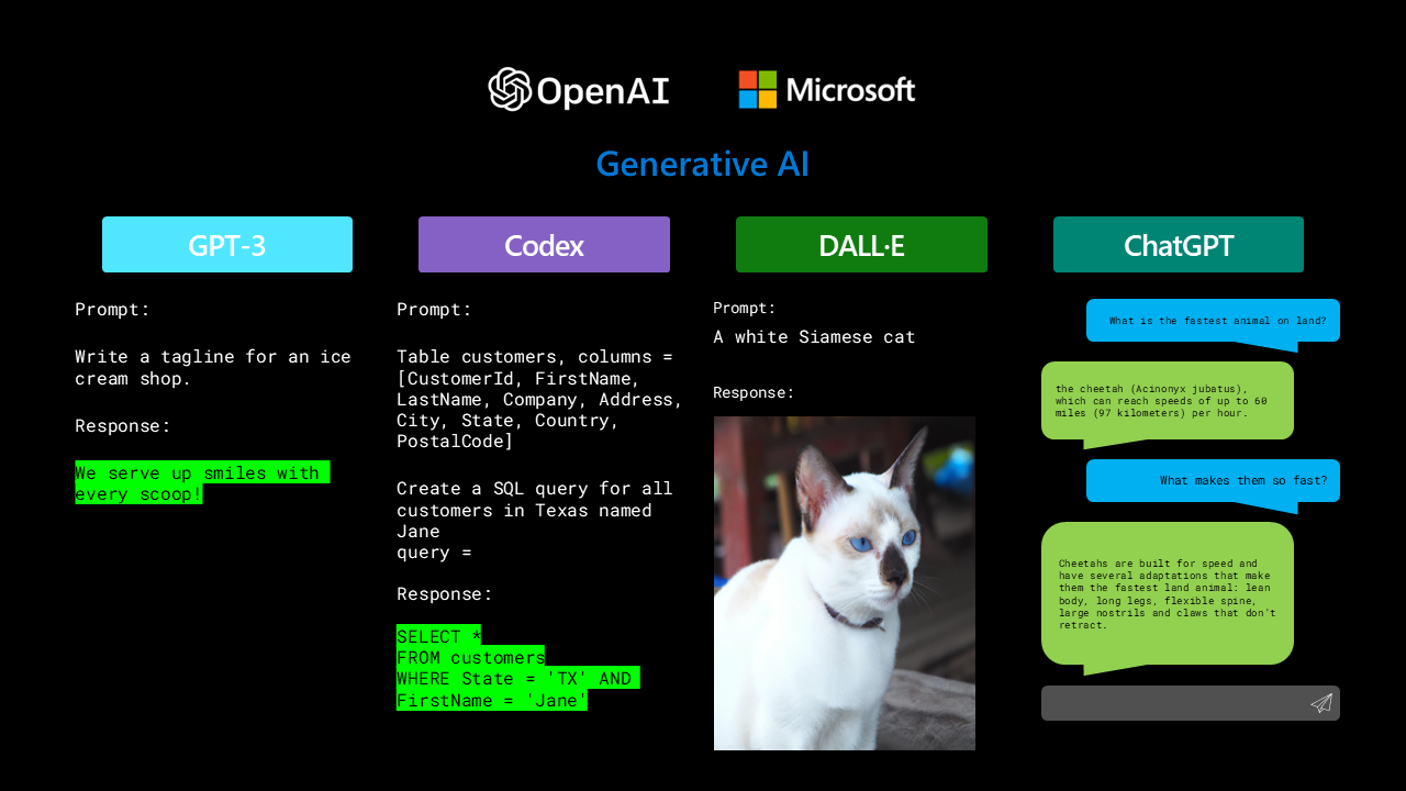
GPT series models, such as GPT-3 and GPT-4 are series of language models developed by OpenAI consisting of some of the largest and most powerful language models to date, with possibly up to 100 trillion parameters in the case of GPT-4 and respectable 175 billion in the case of GPT-3.
GPT-3 is capable of understanding and generating human-like text based on the input it receives. It can perform various tasks, including translation, summarization, question-answering, and even writing code, without the need for fine-tuning. GPT-3’s capabilities have opened up exciting possibilities in natural language processing and have garnered significant attention from the AI community opening it up to mainstream with obvious day-to-day uses.
Building on the success of GPT-3, OpenAI introduced GPT-3.5 and then GPT-4, with each new iteration bringing significant improvements. GPT-3.5 enhanced fine-tuning capabilities and context relevance, while GPT-4, surpassing all previous models, showcases superior complexity and performance. Leveraging the capabilities of GPT-3 like translation, summarization, and code writing, GPT-4 demonstrates heightened understanding and generation of human-like text, expanding the potential applications of AI in various sectors and daily life.
Codex is an AI model built on top of GPT-3, specifically designed to understand and generate code. It can interpret and respond to code-related prompts in natural language and can generate code snippets in various programming languages. The most notable application of Codex is GitHub Copilot, an AI-powered code completion tool developed by GitHub (a Microsoft subsidiary) in collaboration with OpenAI. Copilot assists developers by suggesting code completions, writing entire functions, and even recommending code snippets based on the context of the developer’s current work. Despite its recent legal troubles, it is no doubt a useful tool.
DALL-E is an AI model that combines the capabilities of GPT-3 with image generation techniques to create original images from textual descriptions. By inputting a text prompt, DALL-E can generate a wide array of creative and often surreal images, showcasing the model’s ability to understand the context of the prompt and generate relevant visual representations. DALL-E’s unique capabilities have implications for many creative industries, such as advertising, art, and entertainment, especially when it comes to lowering the entry threshold.
ChatGPT is a AI model fine-tuned specifically for generating conversational responses. It is designed to provide more coherent, context-aware, and human-like interactions in a chat-based environment. ChatGPT can be used for various applications, including customer support, virtual assistants, content generation, and more. By being more focused on conversation, ChatGPT aims to make AI-generated text more engaging, relevant, and useful in interactive scenarios. And while making jokes or understanding Norman McDonald’s humor may be beyond it (so far), the capability is still uncanny.
Microsoft prepared broad range of tools with obvious real-life uses
It is obvious that Microsoft decided to promote AI, seeing the potential to become a main facilitator and infrastructure provider, while also democratizing the whole process and fulfilling its mission of increasing productivity on a global scale. However, during the event it was strongly stated that the partnership with OpenAI, while productive and important, is only part of the range of services offered by Microsoft. The company uses its machine modeling muscles in a variety of ways, presented below, with both old services with AI augmentation and new propositions aimed at increasing productivity.
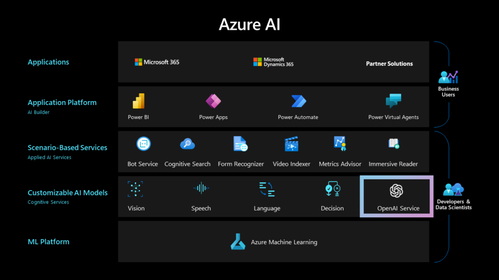
If ChatGPT is all-in-one shop, then Microsoft prepared whole commercial district
Ethics
Now, with figures such as Elon Musk and Bill Gates cautioning against AI and its growth the question of ethics in research and development appears. And while it is rather improbable that ChatGPT, being just a weighed statistical model becomes Roko’s Basilisk – the dangers of automation, unethical data sourcing and increased dependence on quick and easy answers generated by ChatGPT – remain.
So what steps are taken during development of new generation of AI models to ensure that it does more good than bad and won’t go Skynet on the general populace?
Ethical principles: Microsoft has established a set of ethical principles that guide the development and deployment of AI. These principles include fairness, reliability and safety, privacy and security, inclusiveness, transparency, and accountability.
Bias detection and mitigation: Microsoft uses a combination of algorithms and human reviewers to detect and mitigate bias in its AI services. For example, it has developed tools that can identify and correct biased language in chatbots like ChatGPT.
Data privacy and security: Microsoft has strict policies and procedures in place to protect the privacy and security of user data. It also provides users with tools and settings to control how their data is used.
Explainability and transparency: Microsoft aims to make its AI services more explicable and transparent to users. It has developed tools like the AI Explainability 360 toolkit, which allows developers to understand and explain the decisions made by AI models.
Partnerships and collaborations: Microsoft collaborates with governments, NGOs, and academic institutions to ensure that its AI services are used for the social good. For example, it partners with organizations like UNICEF and the World Bank to develop AI solutions that address social and environmental challenges.
Responsible AI initiative: Microsoft has launched a Responsible AI initiative to promote the development and deployment of AI that is ethical, transparent, and trustworthy. The initiative includes a set of tools and resources that developers can use to build responsible AI solutions.
But all of those did not prevent the chatbot from being implicated in a civil libel case filed by Victorian Mayor Brian Hood who claims the AI chatbot falsely describes him as someone who served time in prison as a result of a foreign bribery scandal. Additionally, there are some questions about the regulations about data privacy that may be breached by ChatGPT, which resulted in it being banned in Italy.
The watchdog organization being the bad referred to „the lack of a notice to users and to all those involved whose data is gathered by OpenAI” and said there appears to be „no legal basis underpinning the massive collection and processing of personal data in order to 'train’ the algorithms on which the platform relies”. It is also telling that the AI researcher apologized and committed to working diligently and rebuilding violated trust.
So, while artificial intelligence presents enormous opportunities, and both Microsoft and OpenAI try to conduct their research in an ethical way, it is important to stay informed and watchful about potential dangers and opportunities.
To end the section about Microsoft’s strategy and development of AI products, the most important part must be mentioned – pricing.
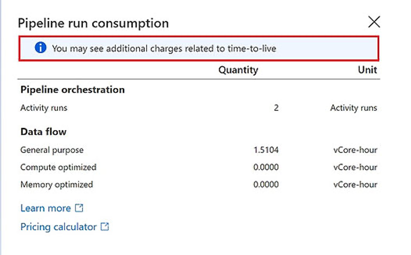
The answer for the questions about using GPT for business is simple – tokenization
The prices itself can and probably will change, as demand stabilizes, but the “pay-as-you-go” model is promising and allows for great flexibility as well as somehow predictable costs. Additionally, there are few AI models to choose from, either focusing on “reasoning” ability or cutting costs.
Summary
All in all, Microsoft’s AI strategy and partnership with OpenAI have the potential to significantly shape the future of AI technology and its applications across various industries. By democratizing AI, integrating AI capabilities into its products, and fostering strategic collaborations, Microsoft is poised to remain at the forefront of the AI revolution, driving innovation and enabling unprecedented advancements in the field. Most importantly for the company, they want users to depend on their productivity increasing services and providers of AI-based solutions to depend on their infrastructure and processing power.
This is a natural extension of Microsoft business strategy, but differently than Azure or Power BI – their hegemony in the AI-sphere is as of now nearly uncontested. Even Google seems to be unable to find the right answer, perhaps because their own AI, Bard, has a habit of providing the wrong ones. For us, mere mortals, all is left to do is keep abreast of developments, hope that ethics prevail during the research and be prepared for a world run with or by AI.
All content in this blog is created exclusively by technical experts specializing in Data Consulting, Data Insight, Data Engineering, and Data Science. Our aim is purely educational, providing valuable insights without marketing intent.


 (+48) 508 425 378
 office@bitpeak.pl
 Tech Drops


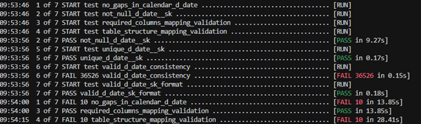
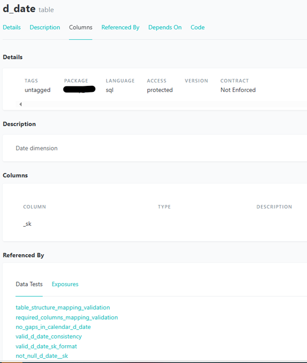


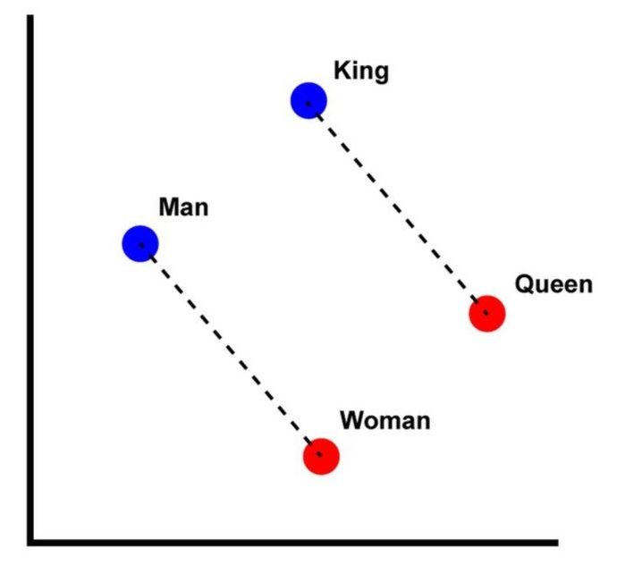 Figure 1 Word embeddings -
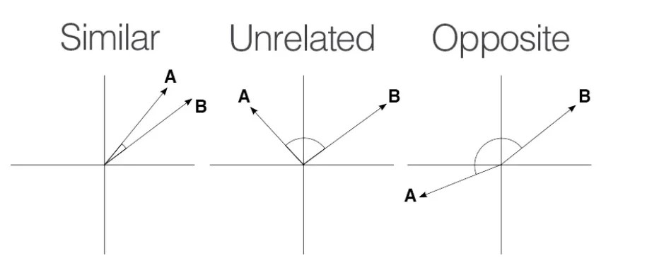
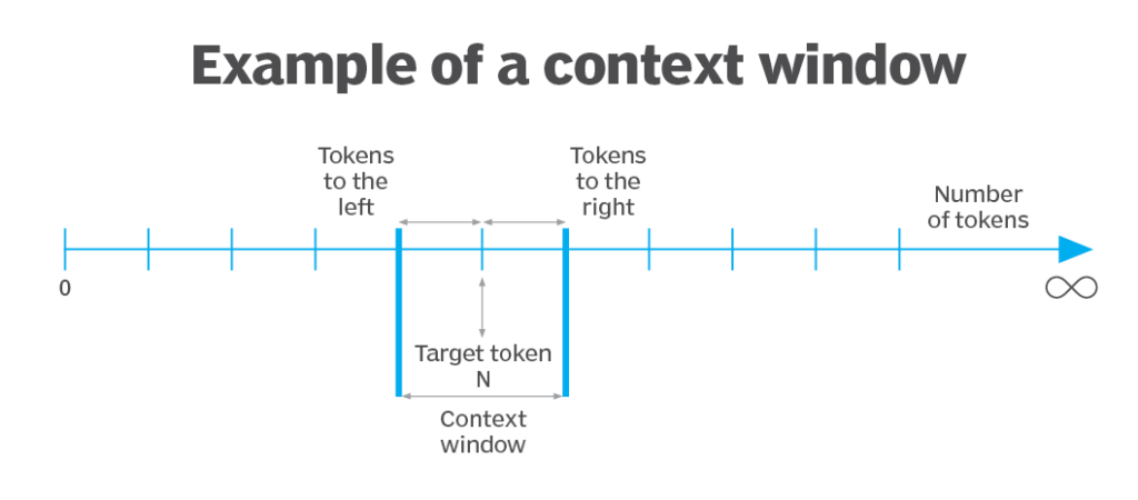
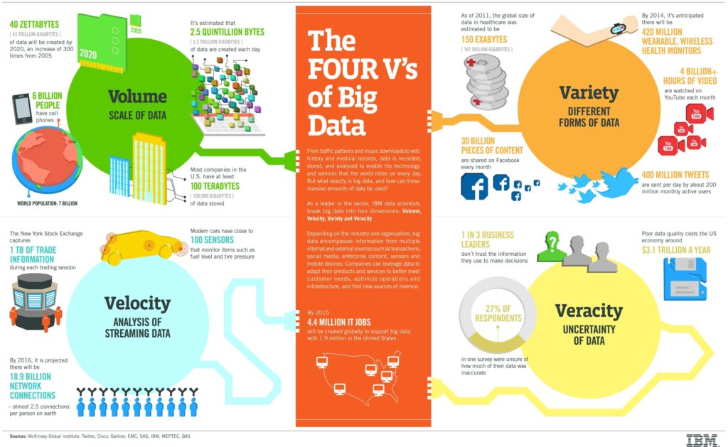 Figure 2. IBM’s infographic on “The Four V’s of Big Data”
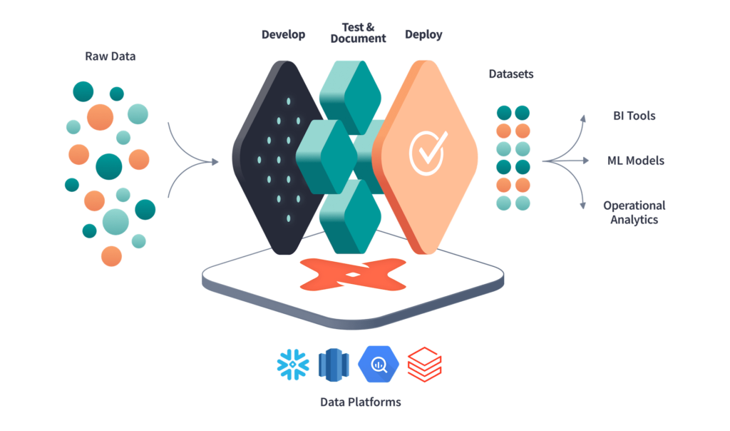 Figure 3. dbt workflow overview
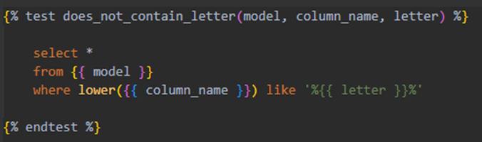
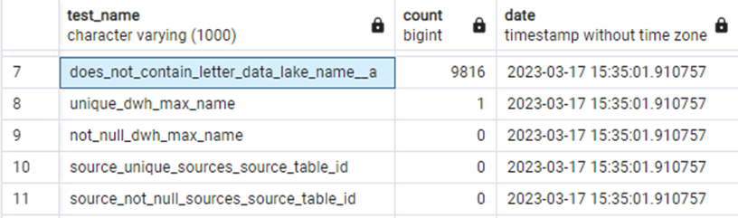 Figure 5. Example of a test summary created through a macro
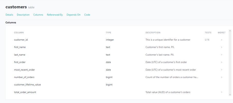 Figure 6. Excerpt from dbt’s documentation of a table
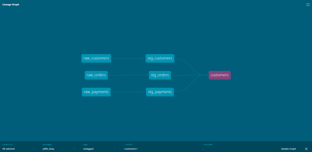 Figure 7. Example of dbt’s lineage graph


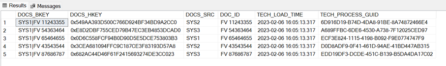 Example BKEY and HKEY:
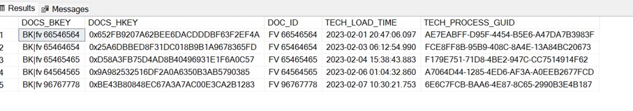 Example HUB structure, description of technical columns one chapter earlier.
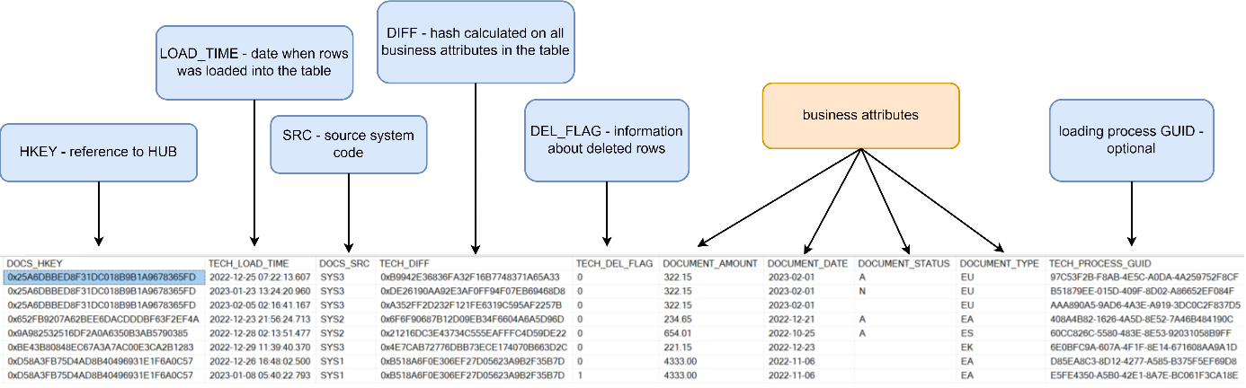 Example of a satellite with data recorded in SCD2 mode:
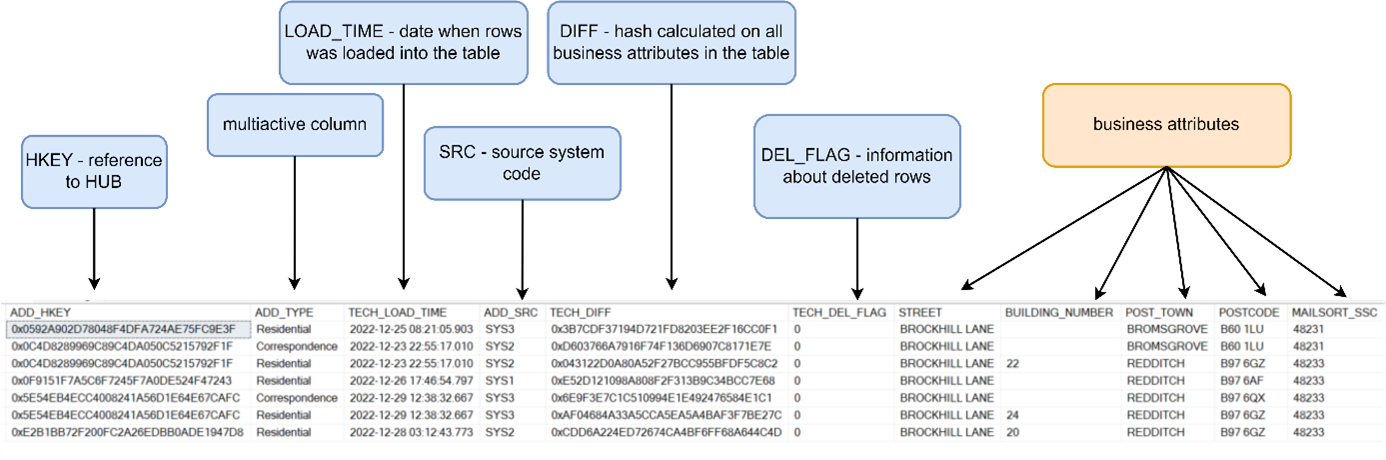 Example of a multiactivity satellite with data recorded in SCD2 mode
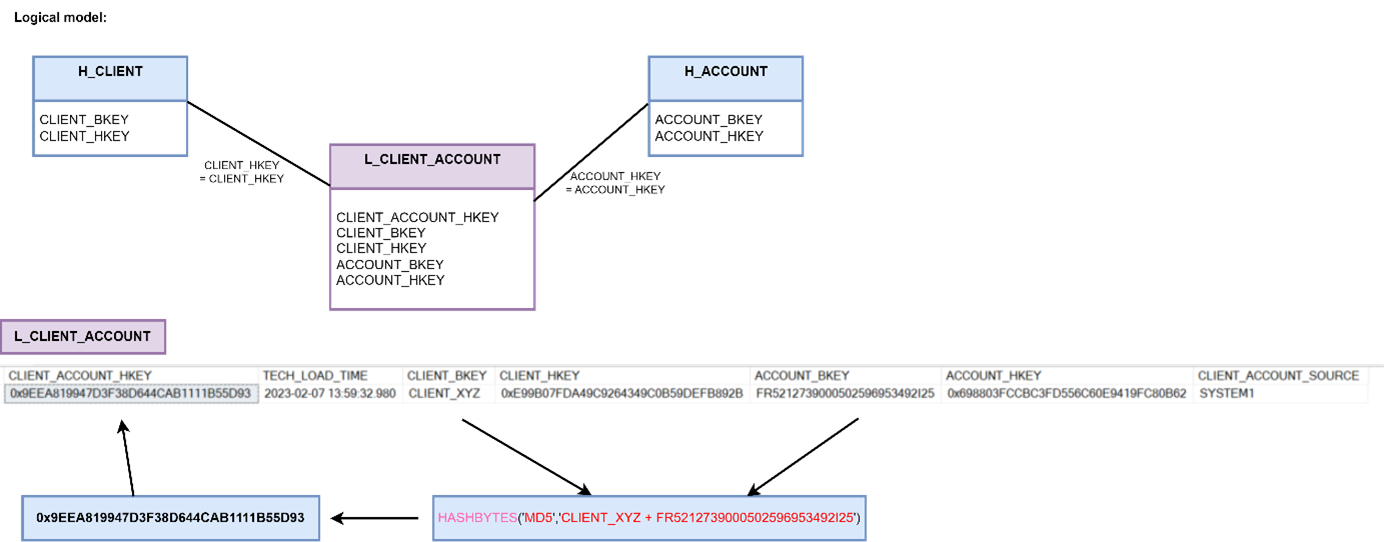
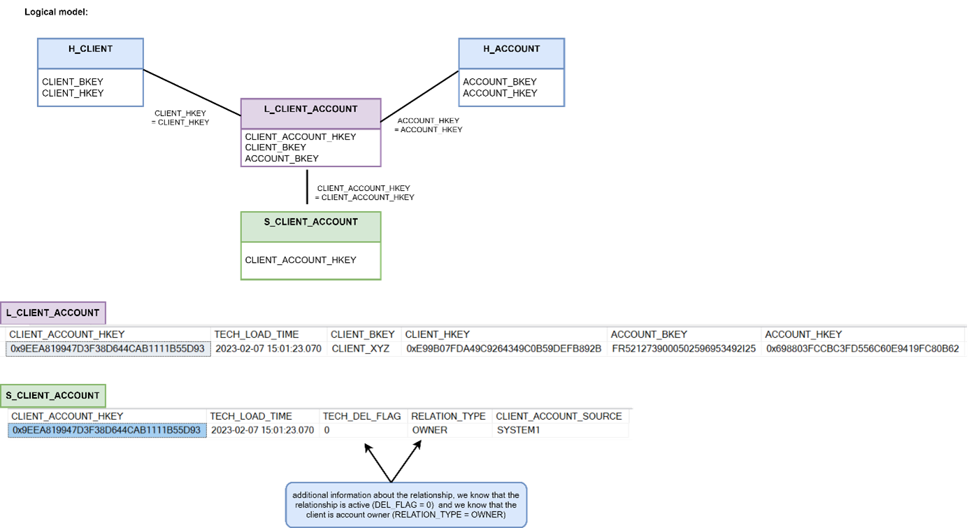
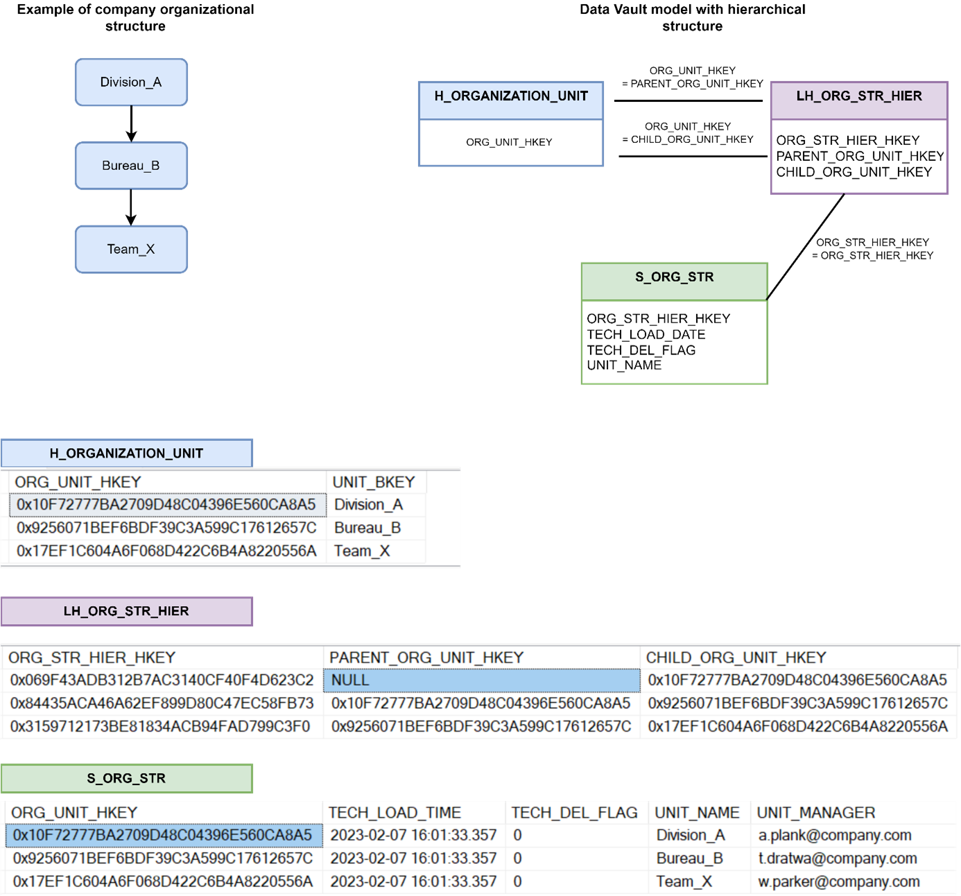 An example of an organisational structure in the Data Vault model using a hierarchical link and an efficiency satellite:
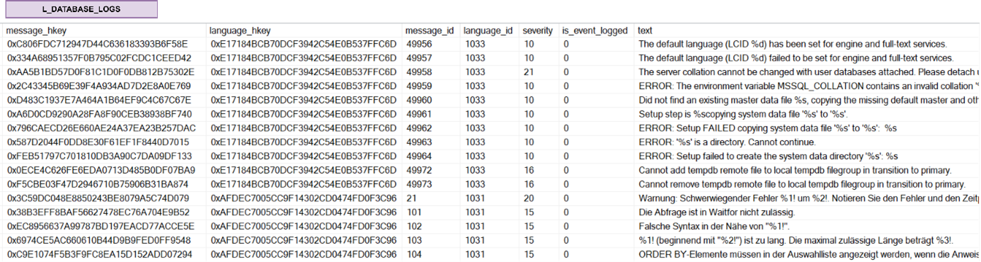 and example of a Non-historicised link
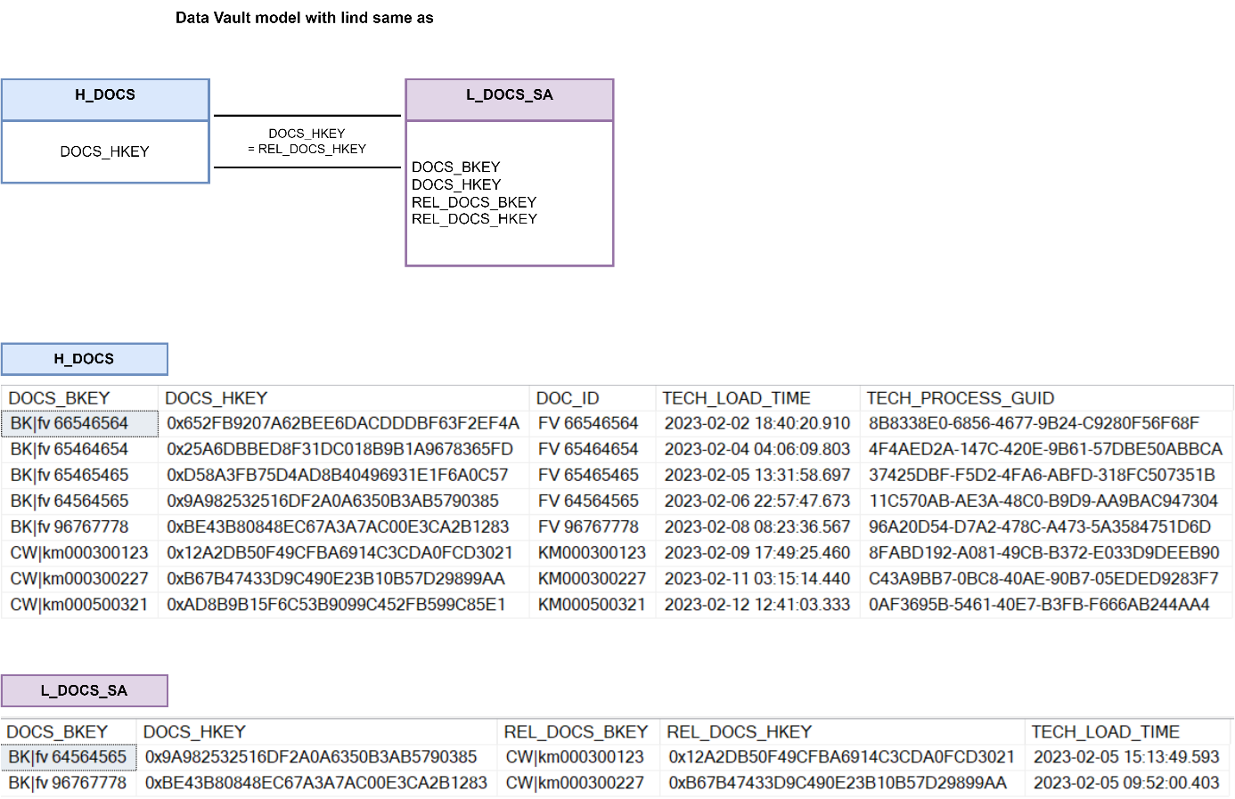 Examples of “same as” link
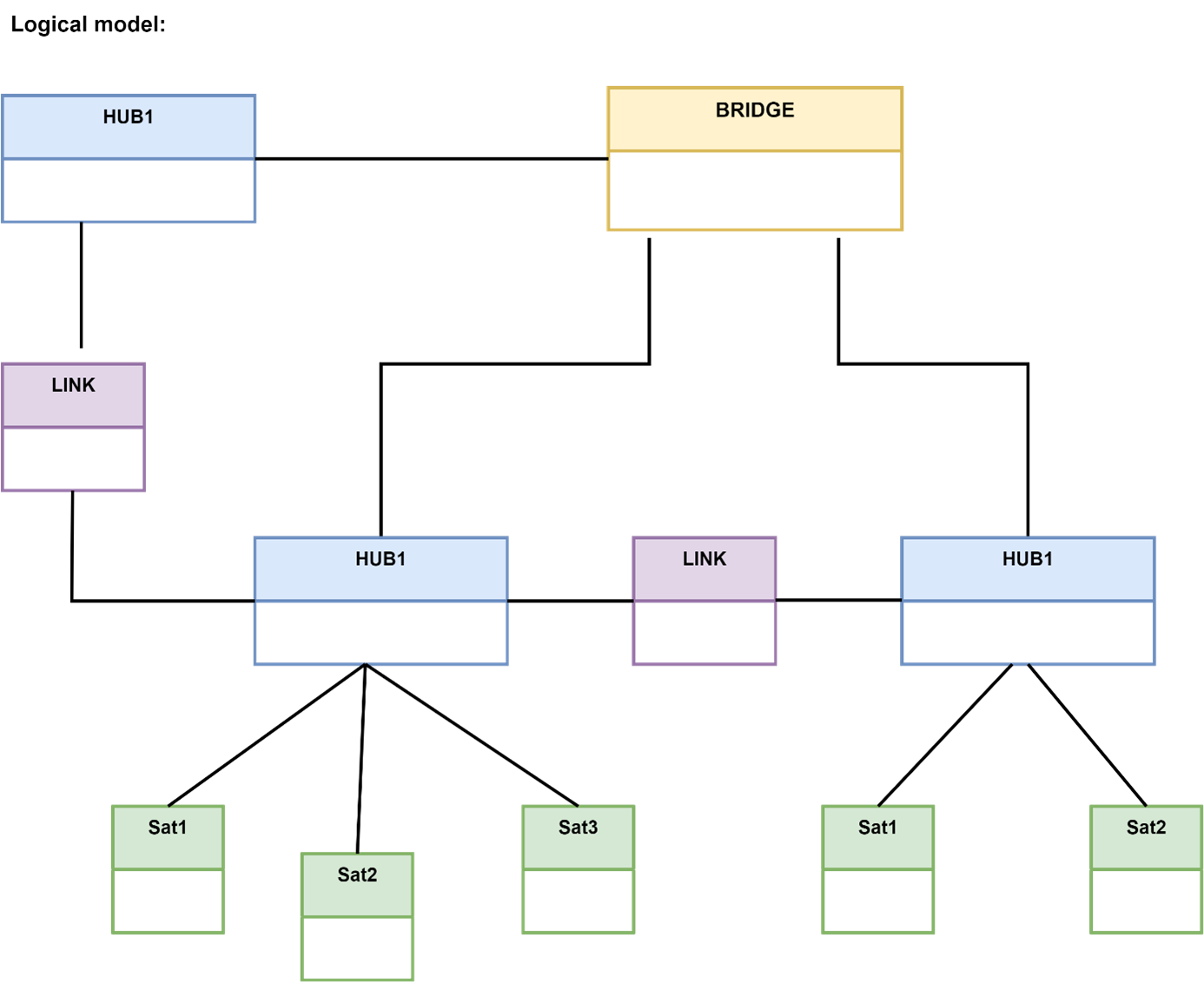

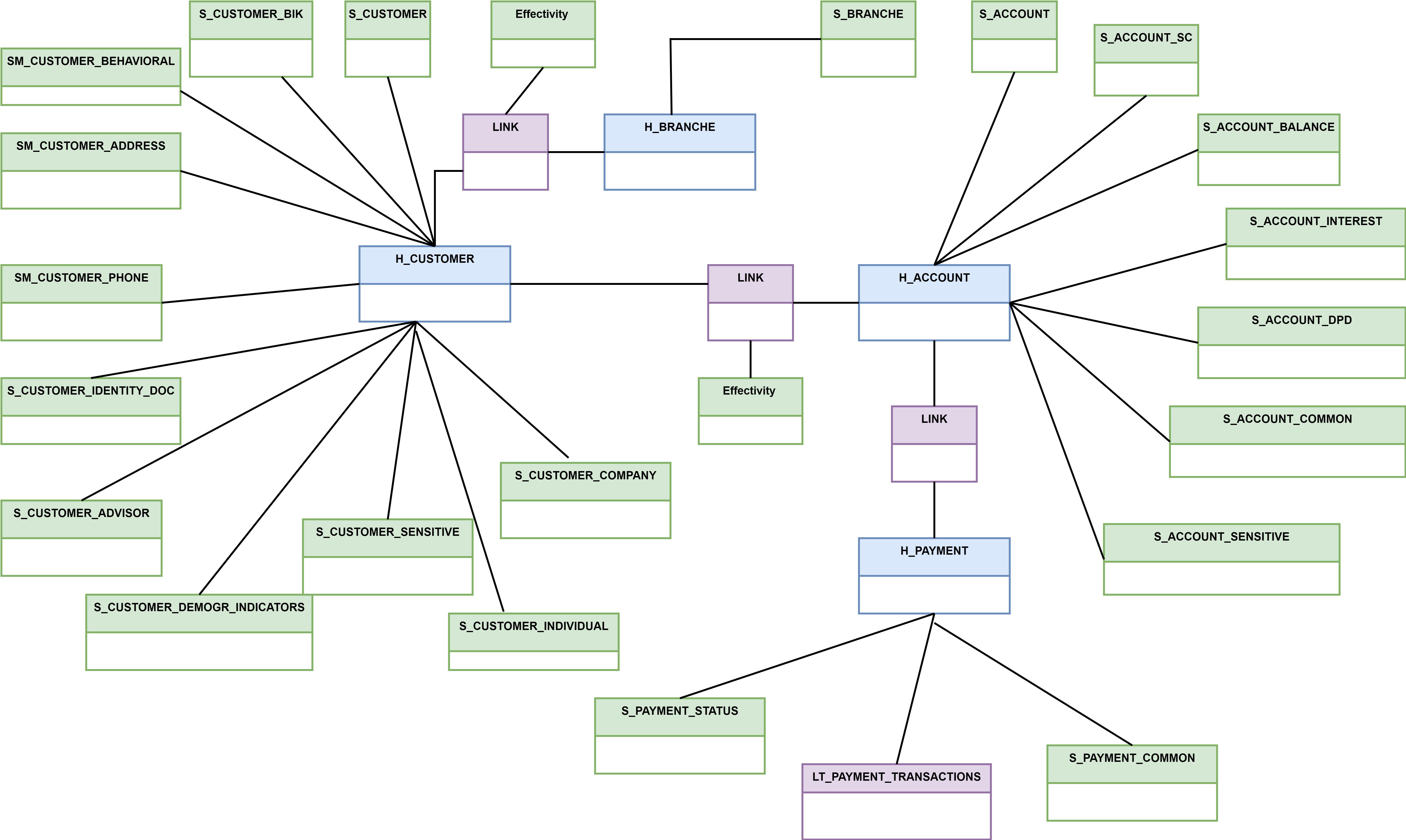


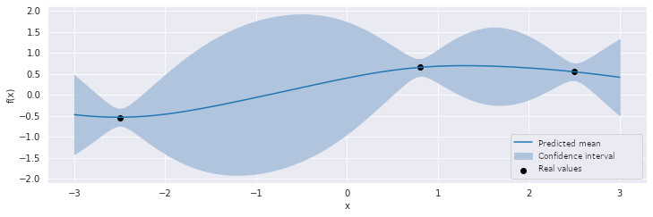 Figure 1: The progression of the surrogate function
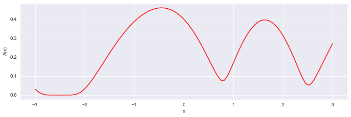 Figure 2: The progression of the acquisition function
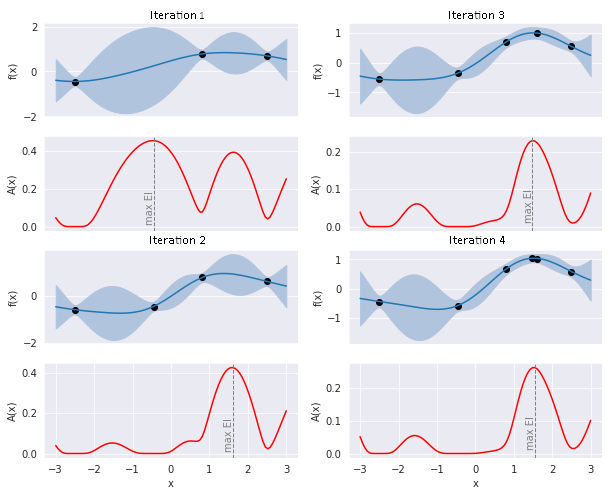
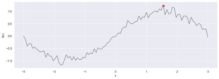 Figure 4: The actual progression of the optimised function


 Pic. 4. Overlaying points from