Smarter Artificial Intelligence with Bayesian Optimization

Introduction

As Artificial Intelligence develops, the need for more and more complex models of machine learning and more efficient methods to deploy them arises. The will to stay ahead of the competition and the interest in the best achievable process automation require implemented methods to get increasingly effective. However, building a good model is not an easy task. Apart from all the effort associated with the collection and preparation of data, there is also a matter of proper algorithm configuration.

This configuration involves inter alia selecting appropriate hyperparameters – parameters which the model is not able to learn on its own from the provided data. An example of a hyperparameter is a number of neurons in one of the hidden layers of the neural network. The proper selection of hyperparameters requires a lot of expert knowledge and many experiments because every problem is unique to some extent. The trial and error method is usually not the most efficient, unfortunately. Therefore some ways to optimise the selection of hyperparameters for machine learning algorithms automatically have been developed in recent years.

The easiest approach to complete this task is grid search or random search. Grid search is based on testing every possible combination of specified hyperparameter values. Random search selects random values a specified number of times, as its name suggests. Both return the configuration of hyperparameters that got the most favourable result in the chosen error metric. Although these methods prove to be effective, they are not very efficient. Tested hyperparameter sets are chosen arbitrarily, so a large number of iterations is required to achieve satisfying results. Grid search is particularly troublesome since the number of possible configurations increases exponentially with the search space extension.

Grid search, random search and similar processes are computationally expensive. Training a single machine learning model can take a lot of time, therefore the optimisation of hyperparameters requiring hundreds of repetitions often proves impossible. In business situations, one can rarely spend indefinite time trying hundreds of hyperparameter configurations in search for the best one. The use of cross-validation only escalates the problem. That is why it is so important to keep the number of required iterations to a minimum. Therefore, there is a need for an algorithm, which will explore only the most promising points. This is exactly how Bayesian optimisation works. Before further explanation of the process, it is good to learn the theoretical basis of this method.

Mathematics on cloudy days

Imagine a situation when you see clouds outside the window before you go to work in the morning. We can expect it to rain during any day. On the other hand, we know that in our city there are many cloudy mornings, and yet the rain is quite rare. How certain can we be that this day will be rainy?

Such problems are related to conditional probability. This concept determines the probability that a certain event A will occur, provided that the event B has already occurred, i.e. P(A|B). In case of our cloudy morning, it can go as P(Rain| Clouds), i.e. the probability of precipitation provided the sky was cloudy in the morning. The calculation of such value may turn out to be very simple thanks to Bayes’ theorem.

Helpful Bayes’ theorem

This theorem presents how to express conditional probability using the probability of occurrence of individual events. In addition to P(A) and P(B), we need to know the probability of B occurring if A has occurred. Formally, the theorem can be written as:

This extremely simple equation is one of the foundations of mathematical statistics [1].

What does it mean? Having some knowledge of events A and B, we can determine the probability of A if we have just observed B. Coming back to the described problem, let’s assume that we had made some additional meteorological observations. It rains in our city only 6 times a month on average, while half of the days start cloudy. We also know that usually only 4 out of those 6 rainy days were foreshadowed by morning clouds. Therefore, we can calculate the probability of rain (P(Rain) = 6/30), cloudy morning (P(Clouds) = 1/2) and the probability that the rainy day began with clouds (P(Clouds|Rain) = 4/6). Basing on the formula from Bayes’ theorem we get:

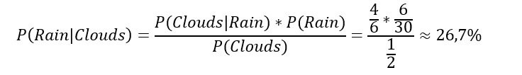
The desired probability is 26.7%. This is a very simple example of using a priori knowledge (the right-hand part of the equation) to determine the probability of the occurrence of a particular phenomenon.

Let’s make a deal

An interesting application of this theorem is a problem inspired by the popular Let’s Make A Deal quiz show in the United States. Let’s imagine a situation in which a participant of the game chooses one of three doors. Two of them conceal no prize, while the third hides a big bounty. The player chooses a door blindly. The presenter opens one of the doors that conceal no prize. Only two concealed doors remain. The participant is then offered an option: to stay at their initial choice, or to take a risk and change the doors. What strategy should the participant follow to increase their chances of winning?

Contrary to the intuition, the probability of winning by choosing each of the remaining doors is not 50%. To find an explanation for this, perhaps surprising, statement, one can use Bayes’ theorem once again. Let’s assume that there were doors A, B and C to choose from. The player chose the first one. The presenter uncovered C, showing that it didn’t conceal any prize. Let’s mark this event as (Hc), while (Wb) should determine the situation in which the prize is behind the doors not selected by the player (in this case B). We look for the probability that the prize is behind B, provided that the presenter has revealed C:

The prize can be concealed behind any of the three doors, so (P(Wb) = 1/3). The presenter reveals one of the doors not selected by the player, therefore (P(Hc) = 1/2). Note also that if the prize is located behind B, the presenter has no choice in revealing the contents of the remaining doors – he must reveal C. Hence (P(Hc|Wb) = 1). Substituting into the formula:

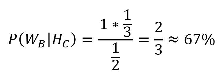
Likewise, the chance of winning if the player stays at the initial choice is 1 to 3. So the strategy of changing doors doubles the chance of winning! The problem has been described in the literature dozens of times and it is known as the Monty Hall paradox from the name of the presenter of the original edition of the quiz show [2].

Bayesian optimisation

As it is not difficult to guess, the Bayesian algorithm is based on the Bayes’ theorem. It attempts to estimate the optimised function using previously evaluated values. In the case of machine learning models, the domain of this function is the hyperparameter space, while the set of values is a certain error metric. Translating that directly into Bayes’ theorem, we are looking for an answer to the question what will the f function value be in the point xₙ, if we know its value in the points: x₁, …, xₙ₋₁.

To visualize the mechanism, we will optimise a simple function of one variable. The algorithm consists of two auxiliary functions. They are constructed in such a way, that in relation to the objective function f they are much less computationally expensive and easy to optimise using simple methods.

The first is a surrogate function, with the task of determining potential f values in the candidate points. For this purpose, regression based on the Gaussian processes is often used. On the basis of the known points, the probable area in which the function can progress is determined. Figure 1 shows how the surrogate function has estimated the function f with one variable after three iterations of the algorithm. The black points present the previously estimated values of f, while the blue line determines the mean of the possible progressions. The shaded area is the confidence interval, which indicates how sure the assessment at each point is. The wider the confidence interval, the lower the certainty of how f progresses at a given point. Note that the further away we are from the points we have already known, the greater the uncertainty.

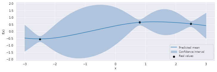Figure 1: The progression of the surrogate function

The second necessary tool is the acquisition function. This function determines the point with the best potential, which will undergo an expensive evaluation. A popular choice, in an acquisition function, is the value of the expected improvement of f. This method takes into account both the estimated average and the uncertainty so that the algorithm is not afraid to „risk” searching for unknown areas. In this case, the greatest possible improvement can be expected at xₙ = -0.5, for which f will be calculated. The estimation of the surrogate function will be updated and the whole process will be repeated until a certain stop condition is reached. The progression of several such iterations is shown in Figure 3.

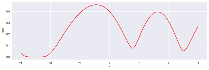Figure 2: The progression of the acquisition function

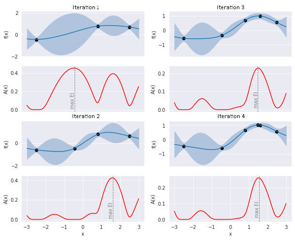
Figure 3: The progression of the four iterations of the optimisation algorithm

The actual progression of the optimised function with the optimum found is shown in Figure 4. The algorithm was able to find a global maximum of the function in just a few iterations, avoiding falling into the local optimum.

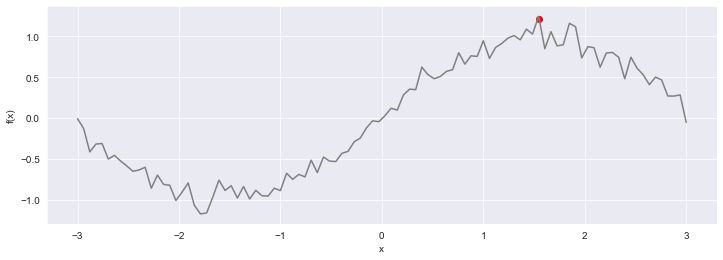Figure 4: The actual progression of the optimised function

This is not a particularly demanding example, but it illustrates the mechanism of the Bayesian optimisation well. Its unquestionable advantage is a relatively small number of iterations required to achieve satisfactory results in comparison to other methods. In addition, this method works well in a situation where there are many local optima [3]. The disadvantage may be the relatively difficult implementation of the solution. However, dynamically developed open source libraries such as Spearmint [4], Hyperopt [5] or SMAC [6] are very helpful. Of course, the optimisation of hyperparameters is not the only application of the algorithm. It is successfully applied in such areas as recommendation systems, robotics and computer graphics [7].

References:

[1] „What Is Bayes’ Theorem? A Friendly Introduction”, Probabilistic World, February 22, 2016. https://www.probabilisticworld.com/what-is-bayes-theorem/ (provided July 15, 2020).
[2] J. Rosenhouse, „The Monty Hall problem. The remarkable story of math’s most contentious brain teaser”, January. 2009.
[3] E. Brochu, V. M. Cora, i N. de Freitas, „A Tutorial on Bayesian Optimization of Expensive Cost Functions, with Application to Active User Modeling and Hierarchical Reinforcement Learning”, arXiv:1012.2599 [cs], December. 2010
[4] https://github.com/HIPS/Spearmint
[5] https://github.com/hyperopt/hyperopt
[6] https://github.com/automl/SMAC3
[7] B. Shahriari, K. Swersky, Z. Wang, R. P. Adams, i N. de Freitas, „Taking the Human Out of the Loop: A Review of Bayesian Optimization”, Proc. IEEE, t. 104, nr 1, s. 148–175, January 2016, doi: 10.1109/JPROC.2015.2494218.
All content in this blog is created exclusively by technical experts specializing in Data Consulting, Data Insight, Data Engineering, and Data Science. Our aim is purely educational, providing valuable insights without marketing intent.